Plotly graphs#

Feature highlight#

The user interface (UI) of a solution app can display both input data (such as strings, integers, floats, and files) and output data (such as 1D/2D/3D graphics, 3D viewers, and images).

In this example, you learn how to:

Write business logic that computes the transcendental butterfly curve with NumPy.
Store the curve data in typed step fields and expose a transaction method that (re)computes it.
Render the data with a Dash dcc.Graph component and customize its layout.
Wire a callback so UI controls trigger the backend computation and refresh the plot.

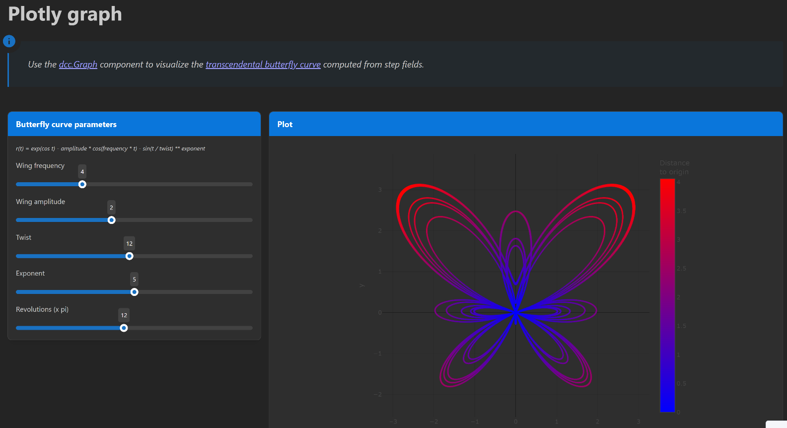
When you complete this example, you can expect the following output in the solution UI:

../../_images/usage_plotly_graph_integration_output.png

Prerequisites#

To render any Plotly-powered data visualization, you need the dcc.Graph component from the Dash Core Components library. For more information, see the Plotly Dash documentation.

Coding#

To display a set of points in a two-dimensional Plotly graph, work through the following sequence of sections.

Logic#

Write the business logic.

Key concept — Business logic

Business logic is plain Python: it has no dependency on SAF and can be developed and tested on its own before it is wired into a step.

Compute the curve coordinates

In the solution/logic folder, the butterfly_curve.py module exposes a compute_butterfly_curve function that generates the set of points of the transcendental butterfly curve for the given parameters.

solution/logic/butterfly_curve.py#

def compute_butterfly_curve(
    wing_frequency: float = 4.0,
    wing_amplitude: float = 2.0,
    twist: float = 12.0,
    exponent: int = 5,
    revolutions: float = 12.0,
    points: int = 10000,
) -> tuple[list[float], list[float], list[float]]:
    """
    Compute the coordinates of the transcendental butterfly curve.

    The curve is defined in polar-like form by

    .. math::

        r(t) = e^{\\cos t} - a \\cos(f t) - \\sin^{n}(t / \\tau)

    with :math:`x = r(t) \\sin t` and :math:`y = r(t) \\cos t`, where :math:`a` is the wing
    amplitude, :math:`f` the wing frequency, :math:`n` the exponent and :math:`\\tau` the
    twist. The default values reproduce the curve described at
    https://en.wikipedia.org/wiki/Butterfly_curve_(transcendental).

    Parameters
    ----------
    wing_frequency : float, default: 4.0
        Frequency of the cosine term that shapes the wings. Higher values add wings.
    wing_amplitude : float, default: 2.0
        Amplitude of the cosine term that shapes the wings. A value of ``0`` removes them.
    twist : float, default: 12.0
        Divider of the parameter in the sine term that twists the wings. It cannot be zero.
    exponent : int, default: 5
        Exponent applied to the sine term. An integer is required because the sine term
        takes negative values.
    revolutions : float, default: 12.0
        Number of half-turns to draw. The parameter ``t`` spans ``[0, revolutions * pi]``.
        The curve is closed for even values.
    points : int, default: 10000
        Number of points used to discretize the curve.

    Returns
    -------
    tuple[list[float], list[float], list[float]]
        Three lists of ``points`` values:

        - the ``x`` coordinates of the curve,
        - the ``y`` coordinates of the curve,
        - the distance of each point to the origin, that is ``sqrt(x ** 2 + y ** 2)``.

    Raises
    ------
    ValueError
        If ``twist`` is zero or if ``exponent`` is not an integer.

    Examples
    --------
    >>> x, y, distance = compute_butterfly_curve(points=5)
    >>> len(x), len(y), len(distance)
    (5, 5, 5)
    """
    if twist == 0:
        raise ValueError("The twist parameter cannot be zero.")
    if exponent != int(exponent):
        raise ValueError("The exponent parameter must be an integer.")

    t = np.linspace(0, revolutions * np.pi, points)
    r = np.exp(np.cos(t)) - wing_amplitude * np.cos(wing_frequency * t) - np.sin(t / twist) ** int(exponent)
    x = r * np.sin(t)
    y = r * np.cos(t)

    return x.tolist(), y.tolist(), np.abs(r).tolist()

Backend#

Create the solution definition.

Key concept — Typed field

A field is a class attribute with a type annotation and a default value. SAF uses the annotation to persist the field, expose it through the REST API, and surface it to the frontend through the DashClient.

Key concept — Transaction method

A transaction method is the only place where step fields are read and written. Any method that touches a field must be decorated with @transaction, which declares the fields it downloads (reads) and uploads (writes) through its StepSpec.

Important

This example deliberately uses a blocking transaction method rather than a long-running one. The business logic was tested beforehand and computes the curve in less than a second, so blocking the UI for that duration is safe and keeps the code simpler.

Nothing prevents you from converting it to a long-running transaction method by adding the @long_running decorator if your own computation takes longer. For more information, see Long-running transaction streaming events.

Frontend#

Expose the solution definition in the UI.

Key concept — Figure layout

The layout key of a Plotly figure controls its size, axes and margins. Plotly enables many kinds of customization. For more information, see its documentation.

Key concept — Callback

A callback is a Dash-decorated function that fires in response to a UI event. In a SAF solution, callbacks reach the backend through project.steps.<step_name>, read or write fields, and invoke transaction methods. No manual HTTP calls are needed.

Trigger the backend computation from the frontend

Write a callback that updates the curve parameter fields, invokes compute_butterfly_curve, and refreshes the figure with the new coordinates.

ui/pages/basic/plot_page.py#

@callback(
    Output("graph", "figure"),
    Output("graph_loading", "visible", allow_duplicate=True),
    Input("butterfly_wing_frequency", "value"),
    Input("butterfly_wing_amplitude", "value"),
    Input("butterfly_twist", "value"),
    Input("butterfly_exponent", "value"),
    Input("butterfly_revolutions", "value"),
    State("url", "pathname"),
)
def draw_butterfly_curve(
    wing_frequency: float,
    wing_amplitude: float,
    twist: float,
    exponent: float,
    revolutions: float,
    project: ExamplesSolution,
) -> tuple[dict, bool]:
    """
    Compute the butterfly curve and refresh the figure.

    On the initial call, the curve is computed with the parameters already stored in the
    step. On any other call, the values of the sliders are written to the step fields
    before the ``compute_butterfly_curve`` transaction method is invoked.

    Parameters
    ----------
    wing_frequency : float
        Value of the wing frequency slider.
    wing_amplitude : float
        Value of the wing amplitude slider.
    twist : float
        Value of the twist slider.
    exponent : float
        Value of the exponent slider. It is cast to an integer for the step field.
    revolutions : float
        Value of the revolutions slider.
    project : ExamplesSolution
        Solution instance injected by the ``DashClient`` from the URL of the page.

    Returns
    -------
    tuple[dict, bool]
        The figure of the computed curve and ``False`` to hide the loading overlay.
    """
    step = project.steps.basic_step

    if ctx.triggered_id is None and not step.distance:
        print("Computing butterfly curve for the first time...")
        step.compute_butterfly_curve()
    else:
        print(
            f"Computing butterfly curve for parameters: wing_frequency={wing_frequency}, "
            f"wing_amplitude={wing_amplitude}, twist={twist}, exponent={exponent}, revolutions={revolutions}"
        )
        step.butterfly_wing_frequency = wing_frequency
        step.butterfly_wing_amplitude = wing_amplitude
        step.butterfly_twist = twist
        step.butterfly_exponent = int(exponent)
        step.butterfly_revolutions = revolutions
        step.compute_butterfly_curve()

    print(f"Computed butterfly curve with {len(step.x_coords)} points.")
    return _butterfly_figure(step), False

Now that your implementation is complete, continue to the Testing section.

Testing#

Finally, test your implementation to confirm it works as expected.

Run the solution and compare your results with the results shown in the Feature highlight section.